Calculate the adjacency spectral embedding of a network.
Arguments
- network
An igraph object with \(n\) nodes.
- d
number of latent dimensions to embed the node positions in.
Value
An \(n\)-by-\(d\) matrix where the \(i^{th}\) row of the matrix corresponds to node \(i\)'s position in the d-dimensional latent space.
Bootstrap samples will retain vertex names of the input network but will loose all other vertex and edge attributes.
Details
This calculates the latent positions of the nodes of a network in \(\mathbb{R}^d\) using adjacency spectral embedding (Sussman et al. 2012) .
Let \(\boldsymbol{A}\) be the adjacency matrix of network with \(n\) nodes.
Additionally, let \(\hat{\boldsymbol{\Lambda}} \in \mathbb{R}^{d \times d}\)
be the diagonal matrix formed by the top d largest-magnitude eigenvalues
of the adjacency matrix and \(\hat{\boldsymbol{U}} \in \mathbb{R}^{n \times d}\)
be the matrix with the corresponding eigenvectors as its columns.
The adjacency spectral embedding of \(\boldsymbol{A}\) is
\(\hat{\boldsymbol{X}} = \hat{\boldsymbol{U}}\hat{\boldsymbol{\Lambda}}^{1/2} \in \mathbb{R}^{n \times d}\).
The \(\text{i}^{\text{th}}\) row of \(\hat{\boldsymbol{X}}\) corresponds to the
location of the \(\text{i}^{\text{th}}\) node in the d dimensional latent space.
References
Sussman DL, Tang M, Fishkind DE, Prieb CE (2012). “A consistent adjacency spectral embedding for stochastic blockmodel graphs.” Journal of the American Statistical Association, 107(499), 1119--1128.
Examples
library(igraph)
#>
#> Attaching package: ‘igraph’
#> The following objects are masked from ‘package:stats’:
#>
#> decompose, spectrum
#> The following object is masked from ‘package:base’:
#>
#> union
data("karate")
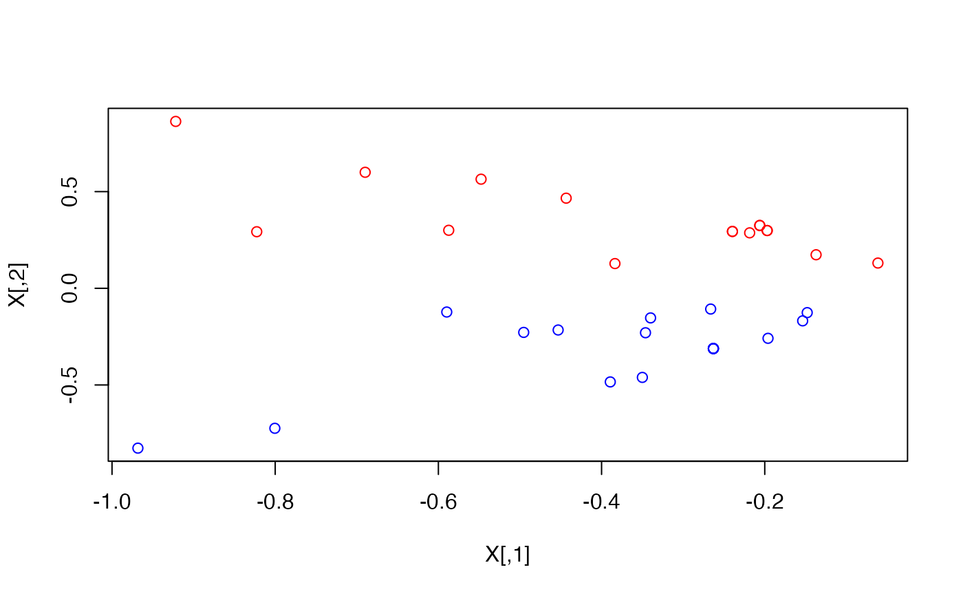
#Find the latent positions in 2D
X <- ASE(karate, 2)
plot(X)
 # Color According to faction
plot(X, col = ifelse(V(karate)$Faction == 1, "red", "blue"))
# Color According to faction
plot(X, col = ifelse(V(karate)$Faction == 1, "red", "blue"))
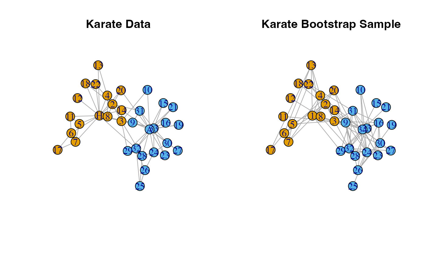
 # Latent Space Bootstrap
set.seed(1)
boot.sample <- bootstrap_latent_space(karate, d = 2, B = 1)
#plot comparison of original data and bootstrap sample
par(mfrow = c(1, 2))
l <- igraph::layout_nicely(karate)
plot(karate,
layout = l,
main = "Karate Data")
plot(boot.sample[[1]],
layout = l,
main = "Karate Bootstrap Sample",
vertex.label = 1:gorder(karate),
vertex.color = V(karate)$color)
# Latent Space Bootstrap
set.seed(1)
boot.sample <- bootstrap_latent_space(karate, d = 2, B = 1)
#plot comparison of original data and bootstrap sample
par(mfrow = c(1, 2))
l <- igraph::layout_nicely(karate)
plot(karate,
layout = l,
main = "Karate Data")
plot(boot.sample[[1]],
layout = l,
main = "Karate Bootstrap Sample",
vertex.label = 1:gorder(karate),
vertex.color = V(karate)$color)