Equivalence Test of Two CDFs Using Mallows Distance

Conduct the equivalence test of two CDFs using the \(p^{\text{th}}\) Mallows distance proposed by Munk and Czado (1998)

Usage

mallows_equiv_test(vec1, vec2, alpha, delta0, sig.level = 0.05)

Arguments

vec1: A numeric vector.
vec2: A numeric vector of the same length as vec1.
alpha: Trimming parameter \(\alpha \in(0, 0.5)\) for trimmed Mallows' distance.
delta0: Tolerance value for hypothesis test.
sig.level: Significance level of the test. Default is 0.05.

Value

A list with the results of the test:

dist.hat is the estimated trimmed Mallows distance between the two distributions, \(\Psi_{\alpha, 2}(\hat{F}, \hat{G})\).
sd.hat is the estimate of the standard deviation between the two distributions, \(\hat{\sigma}_{\alpha}\).
test.stat is the test statistic.
pval is the p-value of the test.
test.result is "REJECT NULL" if pval\(\leq\)sig.level and "FAIL TO REJECT NULL" otherwise.
ci is the upper (1-sig.level) confidence interval for the square of dist.hat
alpha is the trimming parameter used in the test. Sometimes this is slightly different than the input alpha. This test requires an integer \(a\) such that \(\alpha = a/n\). This alpha is the smallest \(\alpha\) that makes this equation true. See Munk and Czado (1998) for details.
delta0 is the tolerance parameter used for the test. This is the same as the input delta0.

Details

This is the equivalence test of two CDFs using the trimmed Mallows distance proposed by Munk and Czado (1998) .

Say \(X_i \overset{iid}{\sim} F\) and \(Y_j \overset{iid}{\sim} G\) for \(i,j = 1, ..., n\) where \(F\) and \(G\) are continuous distribution functions. Let \(\hat{F}_n(x) = \frac{1}{n}\sum_{i=1}^n \boldsymbol{1}\{X_i \leq x\}\) denote the empirical cumulative distribution function (ECDF) of \(X\), and \(\hat{F}^{-1}_n(t) = \inf\{x : F_n(x) \geq t\}\) denote the quantile function. Define \(\hat{G}_m(y)\) and \(\hat{G}^{-1}_m(t)\) similarly for \(Y\).

The Trimmed \(p^{th}\) Mallows distance with trimming parameter \(\alpha \in [0, 1/2)\) is : \(\begin{equation} \Psi_{\alpha, p}(F, G) = \frac{1}{1-2\alpha} \left[ \int_{\alpha}^{1-\alpha} | F^{-1}(u) - G^{-1}(u) | ^p du \right]^{1/p}. \end{equation} \)

Munk and Czado (1998) conduct the equivalence test for some suitable \(0<\Delta_0\in \mathbb{R}\): \( \begin{equation} H_0: \Psi_{\alpha, 2}(F, G) \geq \Delta_0 \quad \text{versus} \quad H_A: \Psi_{\alpha, 2}(F, G) < \Delta_0 \end{equation} \)

Then, a consistent level \(\alpha^*\) test for this hypothesis rejects \(H_0\) if, \( \begin{equation}\label{eqn:MallowTest} \left(\frac{nm}{n+m}\right)^{1/2} \frac{\Psi^2_{\alpha_{n \wedge m}, 2}(\hat{F}_n, \hat{G}_n) - \Delta_0^2}{\hat{\sigma}_{\alpha}(F, G)} \leq q_{\alpha^*} \end{equation} \)

where \(q_{\alpha^*}\) is the \(\alpha^*\) quantile of the standard normal distribution and \(\hat{\sigma}_{\alpha}\) is a consistent estimator of the expected variance between \(F\) and \(G\). See vignette("mallows-equiv-test") or Appendix A of Munk and Czado (1998) for the explicit expression of \(\hat{\sigma}_{\alpha}\).

Currently, this function only runs when \(n=m\). The theory still holds when \(n\neq m\).

See vignette("mallows-equiv-test") for more details on the construction of this test.

Examples

set.seed(2935)
X <- runif(500)
Y <- truncnorm::rtruncnorm(500, a = 0, b = 1, mean = 1/2, sd = 5)

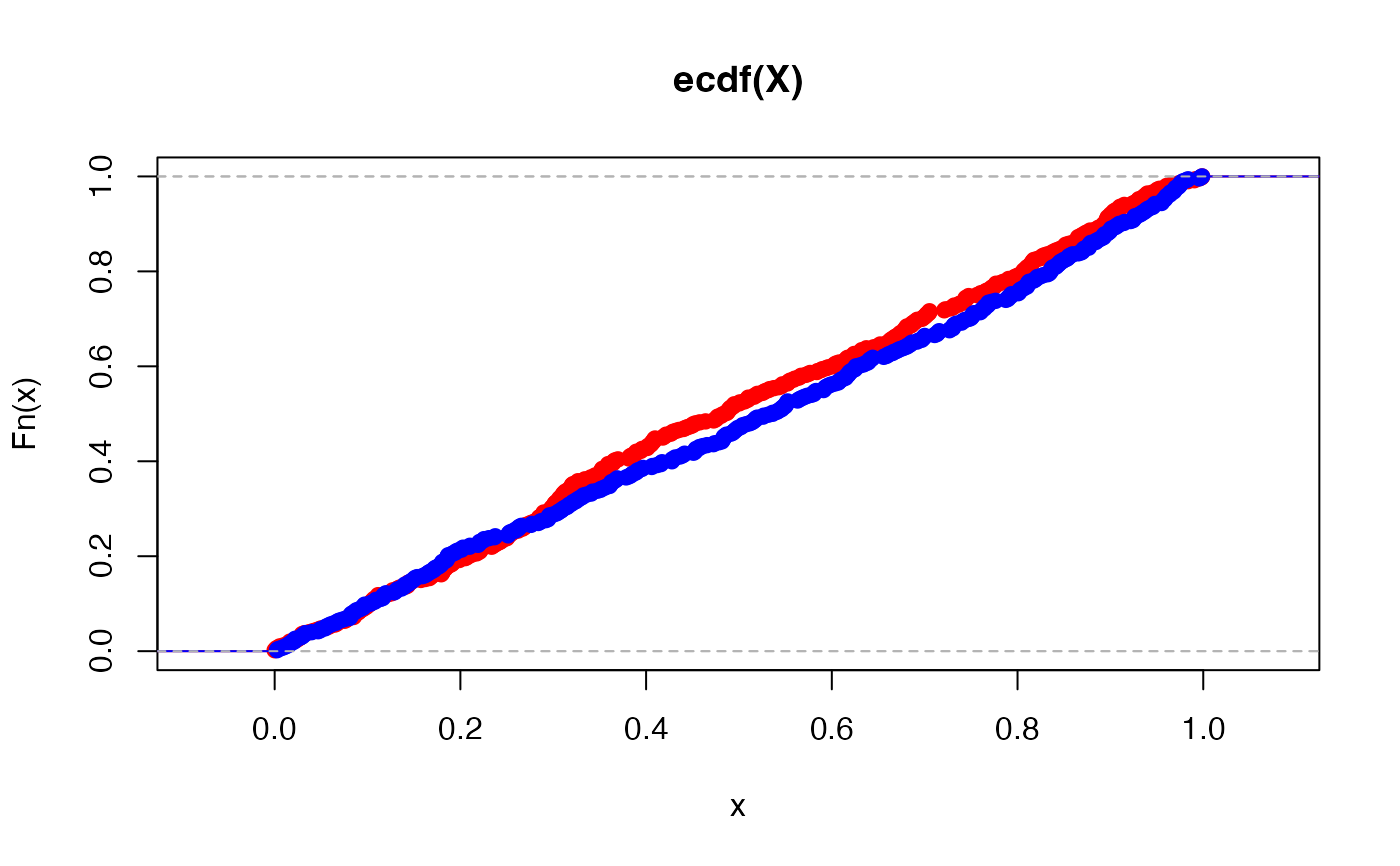
# Plot the ECDFs
plot(ecdf(X), col = "red")
lines(ecdf(Y), col = "blue")


# Run the test for trimming parameter 0.05, tolerance value of 0.8 and
# significance level of 0.05.
test.result <- mallows_equiv_test(X, Y, alpha = 0.05, delta0 = 0.8)
test.result
#> $dist.hat
#> [1] 0.03781523
#> 
#> $sd.hat
#> [1] 0.9830526
#> 
#> $test.stat
#> [1] -10.27074
#> 
#> $pval
#> [1] 4.773456e-25
#> 
#> $test.result
#> [1] "REJECT NULL"
#> 
#> $ci
#> [1] 0.0000000 0.1036966
#> 
#> $alpha
#> [1] 0.05
#> 
#> $delta0
#> [1] 0.8
#>